Tag: jupyter_notebook (Page 14 of 17)

via GIPHY

Roots Magic seems to be a popular tool among genealogists. At least, the Genealogy Guys certainly recommend it.

I’ve been using the tool for about a year now. My previous genealogy database tool seemed to lock away my data in its own proprietary database confining me to the queries and views exposed only in its user interface. Before I switched away, though, I wanted to make sure my next tool would give me a little more latitude with regard to accessing my data. At a genealogy conference in 2017, I actually had a short conversation with the head honcho himself, Bruce Buzbee, and voiced this concern. Bruce briefly mentioned Roots Magic’s connection with sqlite. Interest piqued, I bought his software and made the switch.

It seems like most of the work exploring the sqlite foundation of Roots Magic has been captured at the site SQLiteToolsForRootsMagic. [Side note: Wikispaces, the platform on which SQLiteToolsForRootsMagic is built is going away, so, by the time you read this, the SQLiteTools site might be no more. Fortunately, the site owners are developing migration plans, so stay tuned.] These folks tend to use clients like SQLiteSpy to run their queries. Nothing wrong with that, but since my favorite development canvas lately is Jupyter Notebook, I asked myself, “Self, could you query a Roots Magic database in Jupyter Notebook?” The answer is: absolutely!  Here are some of the steps I took to query a Roots Magic database in Jupyter Notebook.

Step 1: Import the necessary packages

Load all my go-to packages including pandas and matplotlib as well as sqlite3 and Pivotal’s SQL Magic (SQL Magic isn’t necessary, but it makes writing SQL queries a little nicer):

1
2
3
4
5
6
7
8
9
10
import sqlite3

import pandas as pd

import numpy as np

import matplotlib

import matplotlib.pyplot as plt

import matplotlib.style as style



%load_ext sql_magic

%matplotlib inline

plt.style.use('fivethirtyeight')

Step 2: Connect to my Roots Magic file

For demonstration purposes, I grabbed a copy of George Washington’s family tree and saved it off in Roots Magic.  Connecting to the file is pretty darn easy:

1
2
3
4
# Note that sqlite seems to require a full path to the file you wish to load

conn = sqlite3.connect("C:\\data_files\\qsync_laptop\\jupyter_notebooks\\query_gen_dbs\\GeorgeWashingtonFamilyBig.rmgc")

%config SQL.conn_name='conn'  # useful when using sql_magic

cur = conn.cursor()

Step 3: Go to town!

At this point, the only real challenge is dealing with the COLLATE NOCASE issue, but that’s just a minor inconvenience.  After that, it’s just spending time understanding the Roots Magic database schema and the relationships between tables.  SQLiteToolsForRootsMagic has really blazed the trail here, so I encourage you to spend some time on the site looking over the hundreds of posted queries to get a better understanding of the database schema.

With direct access to the database, you can print out facts about your data that may not be exposed in the Roots Magic user interface:

1
2
3
4
5
6
7
8
9
10
11
12
cur.execute("SELECT OwnerID FROM NameTable")

nbr_of_people = len(cur.fetchall())

cur.execute("SELECT FamilyID FROM FamilyTable")

nbr_of_families = len(cur.fetchall())

cur.execute("SELECT FamilyID FROM FamilyTable")

nbr_of_families = len(cur.fetchall())

cur.execute("SELECT FamilyID FROM EventTable")

nbr_of_events = len(cur.fetchall())



print('This database contains {0} individuals.'.format(nbr_of_people))

print('It includes {0} families.'.format(nbr_of_families))

print('It includes {0} events.'.format(nbr_of_events))

Output:

This database contains 529 individuals.
It includes 114 families.
It includes 2679 events.

Or this:

1
2
3
4
5
6
7
8
9
10
11
12
13
14
15
16
17
18
19
20
%%read_sql df_ages -d

SELECT OwnerID

    ,Surname COLLATE NOCASE AS Surname

    ,Given COLLATE NOCASE AS Given

    ,BirthYear AS BirthYear

    ,DeathYear AS DeathYear

    ,(DeathYear - BirthYear) AS age

FROM NameTable n

WHERE COALESCE(BirthYear, 0) > 0 AND COALESCE(DeathYear, 0) > 0

    AND (age BETWEEN 0 AND 110) --remove anyone over 110 years of age or under 0 as that's a likely error



oldest = df_ages.sort_values('age', ascending=False).head(1)

youngest = df_ages.sort_values('age').head(1)

print('This family tree contains {0} individuals with recorded birth and death dates.'.format(df_ages.shape[0]))

print('The oldest person in the tree is {0} {1} at age {2}.'.format(oldest.Given.values[0], oldest.Surname.values[0], 

                                                                   oldest.age.values[0]))

print('The youngest person in the tree is {0} {1} at age {2}.'.format(youngest.Given.values[0], youngest.Surname.values[0], 

                                                                      youngest.age.values[0]))

print('The average age for family members in this tree is {0:.1f} years.'.format(df_ages.age.mean()))

print('The median age for family members in this tree is {0:.1f} years.'.format(df_ages.age.median()))

Output:

This family tree contains 192 individuals with recorded birth and death dates.
The oldest person in the tree is John WASHINGTON at age 99.
The youngest person in the tree is Mildred WASHINGTON at age 1.
The average age for family members in this tree is 52.9 years.
The median age for family members in this tree is 52.0 years.

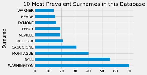
How about some charts?

You can find this work and more on my Github page.